Encoder-decoder
1 Introduction
In graph-based deep learning, low-dimensional vector representations of nodes in a graph are known as node embeddings. The goal of node embeddings is to project graph nodes from their original feature space into a lower-dimensional space to reduce computational complexity while retaining the structural and relational information of nodes in the graph. A key idea in graph-based deep learning, or more precisely in graph representation learning, is to learn these node embeddings.
1.1 Encoder-decoder framework
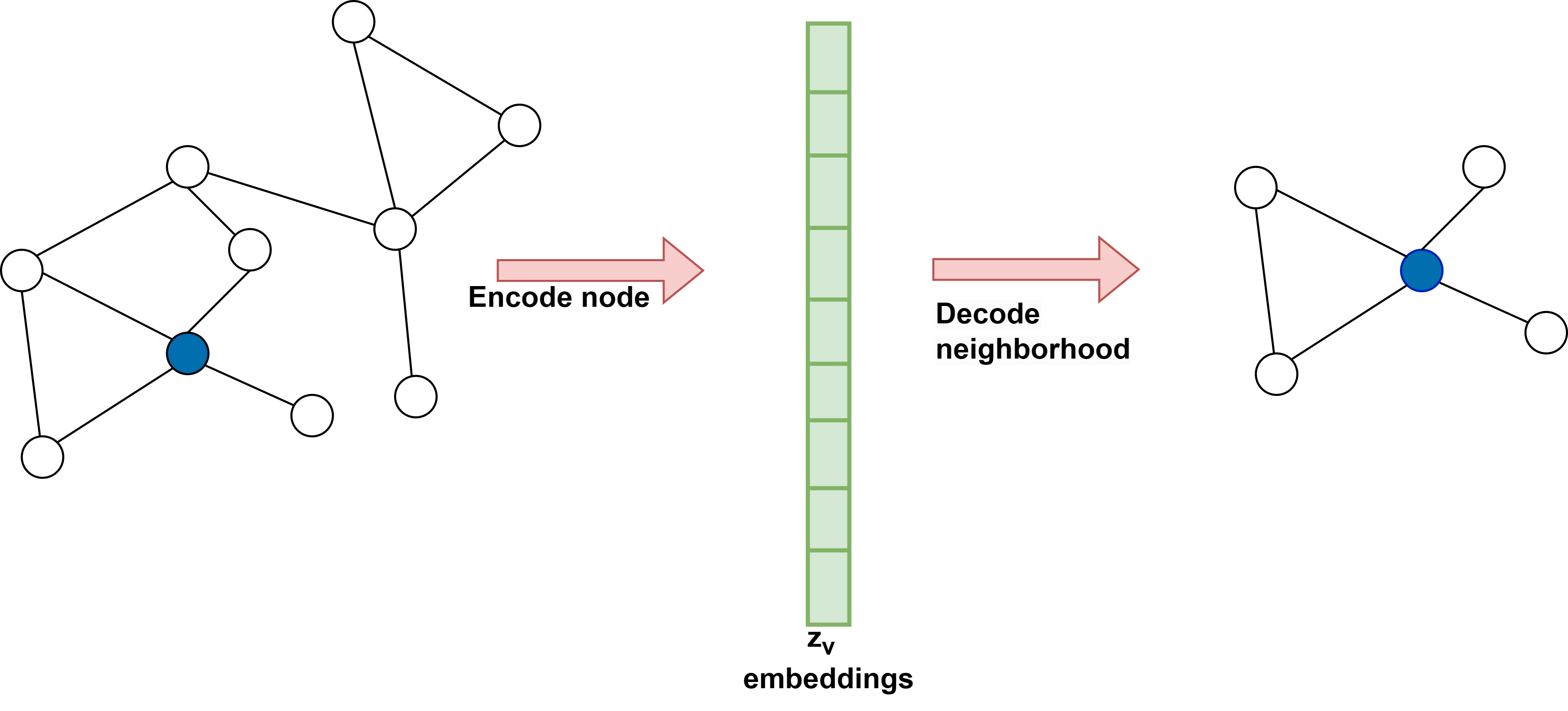
In graph representation learning, we leverage the encoder-decoder framework to facilitate a comprehensive understanding of the graph structure. It is achieved in two crucial steps. Firstly, an encoder model is employed to map each node in the graph to a compact, low-dimensional vector, known as embedding. These embeddings are then passed as input to a decoder model that aims to reconstruct the local neighborhood information for each node in the original graph. By doing so, we obtain a rich and structured graph representation conducive to further analysis. The encoder-decoder framework is depicted in Figure 1.
-
Encoder:
The encoder can be interpreted as a mapping function that transforms node \(v \in V\) in the graph into a vector representation \(Z_v \in \mathbb{R}^d\) where \(Z_v\) represents the embedding for node \(v \in V\). The encoder takes node IDs as input and generates node embeddings corresponding to the node. Hence,
\(ENC: V \to \mathbb{R}^d\)
The encoder typically utilizes a shallow embedding approach, performing an embedding lookup based on the node ID. Shallow embedding approaches are where an encoder that maps each node to a unique embedding is just a simple lookup function without considering any node features. This can be stated as:
\(ENC[v] = Z[v]\)
where matrix \(Z \in \mathbb{R} ^{\left| V \right| \times d}\) is a matrix that contains \(d\)-dimensional embedding vectors for all nodes in the graph and \(Z[v]\) is a row in matrix \(Z\) corresponding to node \(v\). -
Decoder:
The decoder takes as input the node embeddings generated by the encoder and tries to recover graph statistics from these node embeddings.As an illustration, suppose the node embeddings corresponding to node \(v\) is \(z_v\); the decoder may predict a node \(v's\) neighbour set \(N(u)\) or row corresponding to node \(v\) in adjacency matrix of graph \(A[v]\). A simple approach for implementing a decoder is to use pairwise decoders, which try to predict the relationship or similarity between the pair of nodes.Formally it can be stated as:
\(DEC: \mathbb{R}^d \times \mathbb{R}^d \to \mathbb{R}^+\)
Consider an example case where a pairwise decoder is employed to make predictions regarding the adjacency of nodes in the graph. This decoder examines pairs of nodes and predicts whether they are connected by an edge in the graph. Therefore, the relationship between the nodes \(u\) and \(v\) is reconstructed when the pairwise decoder is applied to the pair of their corresponding node embeddings (\(z_u\), \(z_v\)). The ultimate goal of the decoder is to minimize the difference between its output \(DEC(z_u, z_v)\) and the graph-based similarity measure \(S[u,v]\).That is:
\(DEC(ENC(u), ENC(v)) = DEC(z_u, z_v) \sim S[u,v]\)
A common example of a node similarity-based matrix, \(S[u,v]\), is the adjacency matrix, \(A[u,v]\), of the graph.
1.2 Optimization: Reconstructing the graph
To achieve the objective stated in equation 4, the conventional method involves minimizing an empirical reconstruction loss denoted as \(L\). This minimization process occurs over a defined set of training node pairs, denoted as \(D\).:
\(L = \sum_{(u,v) \in D}^{} l(DEC(z_u, z_v), S[u,v])\)
where \(l: \mathbb{R} \times \mathbb{R} \to \mathbb{R}\) quantifies the difference between the estimated similarity value \(DEC(z_u, z_v)\) and true similarity values \(S[u,v]\). The loss function \(l\) might be a mean-squared error or cross-entropy, depending on the decoder and similarity function \(S\).The ultimate aim is to refine the decoder to accurately reconstruct pairwise node relationships in the training set D, typically using stochastic gradient descent or other suitable optimization techniques.
A table of shallow encoding-based Encoder-Decoder approaches is provided below in Table \ref{table 1}.
| Method | Decoder | Loss function |
|---|---|---|
| Laplacian Eigenmaps | \(||z_u - z_v||_2^2\) | \(DEC(z_u, z_v) . S[u,v]\) |
| Graph Factorization | \(z_u^T z_v\) | \(||DEC(z_u, z_v) - S[u,v]||_2^2\) |
| GraRep | \(z_u^T z_v\) | \(||DEC(z_u, z_v) - S[u,v]||_2^2\) |
| DeepWalk | \(e^{z_u^T.z_v} / \sum_{k\in V} e^{z_u^T.z_k}\) | \(-S[u,v]. \log(DEC(z_u, z_v))\) |
| node2vec | \(e^{z_u^T.z_v} / \sum_{k\in V} e^{z_u^T.z_k}\) | \(-S[u,v]. \log(DEC(z_u, z_v))\) |
1.3 Matrix-Factorization approaches to node embeddings
The encoder-decoder concept can be seen through the lens of matrix factorization. The aim is to utilize matrix factorization techniques to obtain a low-dimensional representation capable of capturing a user-defined notion of similarity between nodes. This objective is closely connected to the task of reconstructing elements within a graph’s adjacency matrix. In this study, we will delve into two significant approaches inspired by the matrix factorization technique.
-
Laplacian eigenmaps:
The approach of Laplacian eigenmaps (LE) is based on spectral clustering and is one of the earliest and most influential factorization approaches. In LE approach, the decoder measures the L2 distance between node embeddings.
\(DEC(z_u, z_v) = \parallel z_u - z_v \parallel_2^2\)
The loss function checks the similarity between nodes in the graph and then penalizes embeddings of similar nodes if they are distant.A prominent characteristic of Laplacian eigenmaps is that, when we possess a \(d\) -dimensional embedding denoted as \(z_u\), the optimal solution that minimizes the loss can be obtained by utilizing the \(d\) smallest eigenvectors of the Laplacian matrix (not including the eigenvector corresponding to the 0 eigenvalue).
-
Inner-product methods:
Recent advancements have employed inner-product-based decoders, such as Graph Factorization (GF), GraRep, and HOPE. These decoders perform inner-product on the learned node embeddings using the formula:
\(DEC(z_u, z_v) = z_u^T . z_v\)
While minimizing the loss function:
\(L = \sum_{(u,v) \in D} \parallel DEC(z_u, z_v) - S[u,v] \parallel_2^2\) Here, the assumption is that the inner product between the two learned node embeddings can be seen as a measure of the similarity between them.
1.4 Random walk-based node embeddings
Taking motivation from inner-product approaches, random walk approaches try to adapt the traditional inner-product approach to incorporate stochastic or probabilistic measures of neighborhood overlap. This means that node similarity or neighborhood overlap is not just binary (similar or dissimilar) but probabilistic. The aim is to optimize node embeddings such that nodes that appear frequently together in short graph random walks will have similar embeddings.
Random-walk generation: The first step is to perform a random traversal of graph and generate random walks. The steps can be described as below:
- Let \(G(V, E)\) be a connected graph, and the start node for a random walk is node \(v_0 \in V\).
- Assume that at the \(t\) -th step of random walk, we are at node \(v_t\).
- Then, the next node in random walk will be chosen based on the probability:
\(p(v_{t+1}|v_t) =\) \frac{1}{d(v_t)} , \quad if \quad v_{t+1} \in N(v_t)
0 , \qquad \qquad otherwise \(\)
where \(d(v_t)\) is degree of node \(v_t\) and \(N(v_t)\) denotes the set of neighbour nodes of \(v_t\). In other words, during a random walk, the upcoming nodes are chosen randomly from the current node’s neighbours, and each neighbour has an equal probability of being selected. - To generate random walks that can capture the information about the entire graph, each node is considered the start node for the \(k\) number of random walks. This results in \((N.k)\) random walks in total, where \(N\) is number of nodes in graph. Moreover, every random walk is carried out for a predetermined length, \(l\).
Two approaches based on random walk technique are described below:
- Node2vec:
Node2vec uses the approach of random walk to learn node embeddings for nodes in a graph.Random walks attempt to derive co-occurrence relations between the nodes in a
graph by adopting the notions of centre and context words from the Skip-gram algorithm. The co-occurrence of two nodes in a graph is represented by the tuple (\(v_{cen},
v_{con}\)), where \(v_{cen}\) is the centre (current) node and \(v_{con}\) is one of its context (neighbour) node in the graph.
The process of node2vec can be summarized in the following steps:- For each node in the graph, perform \(k\) random walks of predetermined length, \(l\) on the graph, by following the steps of random walk generation in above section.
- From the random walks, generate a list, \(I\) of the tuples \((v_{cen}, v_{con})\) for the centre and context nodes. It should be noted that a node can play both
roles: centre node and context node. - Two different embeddings will be generated by \(ENCODER\) based on a node’s role as a centre or context node. That is for each node \(v \in V\),
\(ENC(v)_{cen} = Z_{cen}[v]\)
\(ENC(v)_{con} = Z_{con}[v]\) - The decoder model then tries to reconstruct the co-occurrence relationship among nodes by using the information from learned embeddings. That is, the decoder tries to infer the probability of observing a tuple \((v_{cen}, v_{con})\) in \(I\). Formally:
\(DEC(z_{con}, z_{cen}) = \frac{e^{(z_{con})^T.z_{cen}}}{\sum_{k\in V} e^{(z_{con})^T.z_{cen}}}\) - To accurately infer the original graph information from embeddings and match the node co-occurrence information, the DECODER should return high probabilities for
tuples in \(I\) and low probabilities for random tuples. The probability of reconstructing the original \(I\) can be stated as:
\(\prod_{(v_{cen}, v_{con}) \in set(I)}{p(v_{con}|v_{cen})^{\#(v_{con}|v_{cen})}}\)
where \(set(I)\) denotes set of unique tuples in \(I\) and \(\#(v_{con}|v_{cen})\) is the frequency of tuples \((v_{con}|v_{cen})\) in \(I\). Hence, the tuples that are more frequent in \(I\) contribute more to overall probability. - The optimal node embeddings will be learned by minimizing the cross-entropy loss function written as:
\(L = \ - \sum_{(v_{con}|v_{cen}) \in set(I)} \#(v_{con}|v_{cen}). \ log \ p(v_{con}|v_{cen})\)
That is, the objective function is the negative logarithm of equation 12.
- DeepWalk: Study on your own